Billups’ Data Science Team on How Effective Out-Of-Home Advertising Is

Do you wonder how effective Out-Of-Home advertising is from a scientific data driven perspective? A point of view which includes more than data but physical modeling?  Its beyond my comprehension.  The results are not though. 

Billups has its Data Science Team working on quantifying the effectiveness of OOH and much more. Here is their most recent White Paper on Causal Modeling of the Impact of OOH. This is not for the casual reader.  If you didn’t take calculus or statistics at some point in your education, it might be difficult to follow. Not for me though, I took statistics, three times in college. Yes, the same class. 

 

Causal Modeling of the Impact of OOH Media

Randomized control trials in the physical world

Written by Shawn Spooner, Chen Chen, Sicong Chen & Michael Hebert for Billups

 

 

 

 

 

 

Abstract

We consider measuring the ability of out-of-home advertising to drive changes in consumer behaviors, specifically to motivate visits to a physical store. We define the problem as an ensemble of causal models utilizing both a graphical counterfactual model and synthetic controls for the treated audience. We show that a synthetic control that accounts for the spatial/temporal patterns of a subject is highly predictive of future behavior when it models the associated behaviors of closely linked users, and thus is a strong model for establishing the effectiveness of OOH as a treatment.

measuring the ability of out-of-home advertising to drive changes in consumer behaviors, specifically to motivate visits to a physical store.

Introduction

Out-of-Home (OOH) is commonly used to target broad audiences in an attempt to alter the behavioral patterns of its viewers. However, it has been challenging to establish how effective OOH has been in altering the patterns of those who are exposed to the message, due to the enormous number of factors that make up a person’s decision to visit a store, and the high level of difficulty in observing enough covariates to explain a change in the viewer’s patterns of behavior.

establish how effective OOH has been in altering the patterns of those who are exposed to the message, due to the enormous number of factors that make up a person’s decision to visit a store, and the high level of difficulty in observing enough covariates to explain a change in the viewer’s patterns of behavior.

With the ubiquitous use of mobile devices, it has become increasingly possible to create an intricate and varied representation of human movement through the physical world measured down to a meter level of precision. In cataloging this data one can begin to understand the environmental pressures that a person is exposed to over the course of many months and establish strong behavioral groups based on the social structures evident in the data. When observed on a macro level these groups are very predictive of future behavior for members of the community.

Motivated by these challenges we develop a method of causal analysis for estimating the effectiveness of #OOH by combining a massive data set of observations with purchase data, visit history, social, demographic, and psychographic data to build a very thorough picture of the human patterns that allow us to construct a very accurate baseline of behavior.

we develop a method of causal analysis for estimating the effectiveness of #OOH by combining a massive data set of observations with purchase data, visit history, social, demographic, and psychographic data to build a very thorough picture of the human patterns that allow us to construct a very accurate baseline of behavior.

Problem Setup

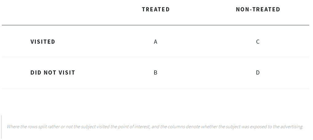
Our method begins by splitting each person into one of four groups for both a pretreatment period and a treatment window. As a practical example, take a bus wrapped with an advertisement for a store that runs a fixed route with set stops. One can observe which devices are present at the same locations and times as the bus, and which are traveling in a path that would allow them to see the message wrapped on the outside of the vehicle. This is done by observing the local trajectory of the device, and analyzing all the obstructions, buildings, and other factors that impair their ability to take in the message. Once a person is marked as treated they can be placed into A if they visit the store in question at least once in the study period, or B if they do not. Visitation is established by aggregating over the devices check-in data, purchase data, and location traces. As the bus is traversing the route it is possible to observe and track all the devices that were nearby but were unable to take in the message, these devices are observed and placed into C if they visit the POI and D if they do not.

It is possible to create a placebo intervention by winding back the clock before the intervention started, by aligning the days of the week and times, then repeating the same assignment procedure. This allows for the discovery of the baseline characteristics of the consumer that led to visitation, as well as observe their propensity to be in the treatment area during the study period.

Visits Graph

Each subject is then augmented with a continuous feature matrix V encoding times of visits, divided into 5-minute buckets of time. A visitation graph can then be induced by linking users who co-visit points of interest at similar times and in similar frequencies. Each node represents a subject, and each edge represents how similar the subject’s visitation patterns are in terms of both frequency and time. The edges are undirected as the relationship to a point of interest is assumed symmetric between subjects when they share the same time window and point of interest. The weight of the edge is determined by how similar the frequency and time of day patterns are between each pair of devices.

This graph is then utilized to create lower dimensional dense vector embeddings using graph2vec that captures the structure of the graph, specifically the neighborhood region surrounding the device.

Causal Modelling

In the following sections, we propose three methods that one can use to accurately establish the causal effect of OOH advertising on the observed visitation patterns of a person to a series of points of interest. The quantity we are attempting to measure is E[YT=1−Y^T=0] which is the estimated treatment effect.

Counterfactual

Addressing the question of what would have happened sans treatment is handled by counterfactual reasoning. We frame this as a probabilistically equivalent audience match between pairs of untreated and treated subjects, minimizing the distance between the pair. Distance is computed using Jaccard distance for categorical data and Mahalanobis distance for continuous data. For persons x and y, where X, Y are the categorical components and

are the continuous features the distance is computed as 

 

                    X is as the high dimensional feature vector indicating which demographic, psychographics, and attitudinal groups this person is a member of, while is formed over the visitation and travel pattern history of this person. We set the similarity of direct neighbors in the friend graph to near zero to prevent sampling persons who are likely friends to control for direct network effects. We then randomly sample among the top 10 matches for each person, to build out controls for each treated user to perform 8-fold cross-validation. Observing the difference in outcomes between the treated and control groups we establish the estimated treatment effect. The less variance there is between the folds, the higher confidence we have in the result not being overly sensitive to the choice of control.

Synthetic Controls

The synthetic control model considers the problem of predicting the probability of visitation by learning a representation from the spatial traces and visitation history of each subject during the pre-treatment period. This method is especially good when it is challenging to disentangle who is exposed to the treatment. The trained model is then used to make predictions about who will visit the store during the study period, this becomes the synthetic control audience. The difference in outcomes between the observed audience and the predicted audience becomes the basis for the estimated treatment effect.

Propensity Matching

Thirdly, we model the probability of treatment and match devices based on their propensity for treatment. This allows for the discovery of the features that are covariates of the treatment. These propensity scores allow us to match subjects with similar probabilities of being treated, and observe the effect of treatment between the two groups, thus breaking the dependence of any confounding X values on the treatment probability. Devices are matched by picking controls that minimize the statement $E(x)-E(y)|$ where E(x) is the expected propensity score. For each treated device we randomly sample closely matched control devices to build out 8-fold cross-validation sets. We then compare the mean difference in outcomes between the two populations as the average treatment effect.

Summary

We introduce a model that takes the input of the three methods above, which has shown a strong ability to disentangle confounding variables, and thus accurately describe the causal relationships between OOH exposure and outcome. We show that one can model this as a causal graph, a simplified version of which is shown below.

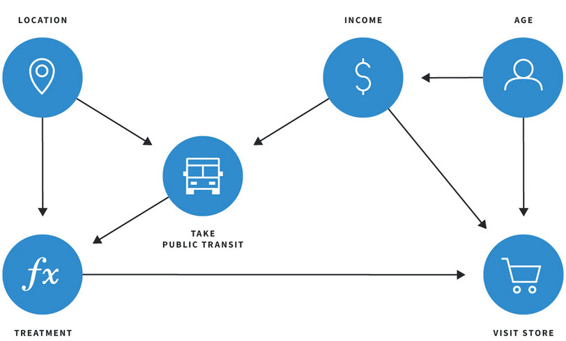
By modeling the problem in these two ways we are able to estimate the causal effect of the treatment, as well as ascertain that the treatment was the cause of the behavior we observed. We phrase the causal graph building as a machine learning task, and learn the graph over the observed data. Future work will consider the challenge of unwinding the effect of repeat exposures, and the attention decay phenomenon we observed in this study.